What is Multidimensional Scaling?

Multidimensional Scaling (MDS) is a dimensionality reduction technique that is useful for exploratory data visualization. Some other popular dimensionality reduction techniques include Principle Component Analysis (PCA) and t-Distributed Stochastic Neighbor Embedding (t-SNE).

Given a similarity matrix (e.g. a distance matrix), MDS projects the data points into an N-dimensional space while minimizing the amount of similarity information lost. In the ideal case, the closer the projected points are to one another, the more similar the are while the farther apart they are, the less similar they are. MDS can reveal similarity patterns in your data that were not previously obvious.

The data 🥚🥓🦐🥞🥗🥗🥕🥓🥔🥐

In this post I’ll be performing MDS on a dataset of the nutritional information for the food emoji and visualizing the result! You can find the dataset on Kaggle here.

First, let’s load in some packages.

library(tidyverse)
library(janitor)
library(knitr)
library(stringi)
library(ggimage)
library(kableExtra)

And for all of these fun inline emojis 🥒🥝🥒🥚…

# install.packages("devtools")
devtools::install_github("hadley/emo")
library(emo)

Next, let’s load in the dataset.

# read in the data
emoji_raw <- read_csv("data/emoji_nutritional_data.csv") %>%
  janitor::clean_names()  # clean up column names

A quick glimpse of the raw data

glimpse(emoji_raw)

## Observations: 58
## Variables: 35
## $ name                  <chr> "grapes", "melon", "watermelon", "tangerine", "…
## $ emoji                 <chr> "\U0001f347", "\U0001f348", "\U0001f349", "\U00…
## $ calories_kcal         <dbl> 0.69, 0.28, 0.30, 0.53, 0.29, 0.89, 0.50, 0.63,…
## $ carbohydrates_g       <dbl> 0.1810, 0.0658, 0.0755, 0.1334, 0.0932, 0.2284,…
## $ total_sugar_g         <dbl> 0.1548, 0.0569, 0.0620, 0.1058, 0.0250, 0.1223,…
## $ protein_g             <dbl> 0.0072, 0.0111, 0.0061, 0.0081, 0.0110, 0.0109,…
## $ total_fat_g           <dbl> 0.0016, 0.0010, 0.0015, 0.0031, 0.0030, 0.0033,…
## $ saturated_fat_g       <dbl> 0.00054, 0.00025, 0.00016, 0.00039, 0.00039, 0.…
## $ monounsaturated_fat_g <dbl> 0.00007, 0.00002, 0.00037, 0.00060, 0.00011, 0.…
## $ polyunsaturated_fat_g <dbl> 0.00048, 0.00039, 0.00050, 0.00065, 0.00089, 0.…
## $ total_fiber_g         <dbl> 0.009, 0.009, 0.004, 0.018, 0.028, 0.026, 0.014…
## $ cholesterol_mg        <dbl> 0, 0, 0, 0, 0, 0, 0, 0, 0, 0, 0, 0, 0, 0, 0, 0,…
## $ vitamin_b6_mg         <dbl> 0.00086, 0.00163, 0.00045, 0.00078, 0.00080, 0.…
## $ vitamin_a_iu          <dbl> 0.66, 0.00, 5.69, 6.81, 0.22, 0.64, 0.58, 0.38,…
## $ vitamin_b12_ug        <dbl> 0e+00, 0e+00, 0e+00, 0e+00, 0e+00, 0e+00, 0e+00…
## $ vitamin_c_mg          <dbl> 0.032, 0.218, 0.081, 0.267, 0.530, 0.087, 0.478…
## $ vitamin_d_iu          <dbl> 0.00, 0.00, 0.00, 0.00, 0.00, 0.00, 0.00, 0.00,…
## $ vitamin_e_iu          <dbl> 0.0019, 0.0005, 0.0005, 0.0020, 0.0015, 0.0010,…
## $ vitamin_k_ug          <dbl> 0.146, 0.025, 0.001, 0.000, 0.000, 0.005, 0.007…
## $ thiamin_mg            <dbl> 0.00069, 0.00015, 0.00033, 0.00058, 0.00040, 0.…
## $ riboflavin_mg         <dbl> 0.00070, 0.00031, 0.00021, 0.00036, 0.00020, 0.…
## $ niacin_mg             <dbl> 0.00188, 0.00232, 0.00178, 0.00376, 0.00100, 0.…
## $ folate_ug             <dbl> 0.02, 0.08, 0.03, 0.16, 0.11, 0.20, 0.18, 0.03,…
## $ pantothenic_acid_mg   <dbl> 0.00050, 0.00084, 0.00221, 0.00216, 0.00190, 0.…
## $ choline_mg            <dbl> 0.056, 0.076, 0.041, 0.102, 0.051, 0.098, 0.055…
## $ calcium_g             <dbl> 0.10, 0.11, 0.07, 0.37, 0.26, 0.05, 0.13, 0.07,…
## $ copper_mg             <dbl> 0.00127, 0.00060, 0.00042, 0.00042, 0.00037, 0.…
## $ iron_mg               <dbl> 0.0036, 0.0034, 0.0024, 0.0015, 0.0060, 0.0026,…
## $ magnesium_mg          <dbl> 0.07, 0.11, 0.10, 0.12, 0.08, 0.27, 0.12, 0.05,…
## $ manganese_mg          <dbl> 0.00071, 0.00035, 0.00038, 0.00039, 0.00030, 0.…
## $ phosphorus_g          <dbl> 0.20, 0.05, 0.11, 0.20, 0.16, 0.22, 0.08, 0.13,…
## $ potassium_g           <dbl> 1.91, 1.82, 1.12, 1.66, 1.38, 3.58, 1.09, 1.09,…
## $ selenium_ug           <dbl> 0.001, 0.004, 0.004, 0.001, 0.004, 0.010, 0.001…
## $ sodium_g              <dbl> 0.02, 0.09, 0.01, 0.02, 0.02, 0.01, 0.01, 0.01,…
## $ zinc_mg               <dbl> 0.0007, 0.0007, 0.0010, 0.0007, 0.0006, 0.0015,…

What are the dimensions?

dim(emoji_raw)

## [1] 58 35

Since there are a quite a few nutritional categories in this dataset, I decided to narrow things down a bit based on the U.S. Food & Drug Administration’s recommendations here.

They recommend limiting total fat, cholesterol, and sodium, and getting more of dietary fiber , vitamin A, vitamin C, calcium, and iron. I decided to add total sugar and protein into the mix as well.

Let’s extract the name and emoji information from the original dataset since we’ll need that later on for plotting.

emoji_info <- emoji_raw %>% 
  select(name, emoji)

Let’s also create a new version of the dataframe with only the nutrients that we are focusing on.

emoji_data <- emoji_raw %>% 
  select(calcium_g, total_fiber_g, vitamin_a_iu, vitamin_c_mg, 
         saturated_fat_g, cholesterol_mg, sodium_g, iron_mg,
         total_sugar_g, protein_g)

MDS

Before we can perform MDS, we need to normalize our data so that our sample means are centered at zero and our sample variances are equal to one. This will take care of any issues of some nutrients being in different units than others. We can normalize our dataset using the scale() function.

emoji_scaled <- scale(emoji_data) %>% 
  as_tibble()

Quick sanity check to make sure everything went as expected:

emoji_scaled %>% 
  summarize_all(var) %>% 
  kable() %>% 
  kable_styling() %>%
  scroll_box(width = "100%")

emoji_scaled %>% 
  summarize_all(mean) %>% 
  kable() %>% 
  kable_styling() %>%
  scroll_box(width = "100%")

Okay, looks good! The next step is to create a distance matrix using dist(). The default distance measure of dist() is euclidean distance. This may not be the best choice for this situation but will be sufficient for the purposes of this post.

emoji_dist <- emoji_scaled %>% 
  dist()

Now we’re reading to perform MDS using cmdscale() from the preloaded stats package. By setting the argument k = 2, we’re telling cmdscale that we want to project our data into a 2D space.

emoji_mds <- cmdscale(d = emoji_dist, k = 2)

emoji_mds %>% 
  head()

##           [,1]        [,2]
## [1,] -1.268054 -0.41890144
## [2,] -1.331595 -0.18949516
## [3,] -1.337405 -0.41653397
## [4,] -1.422334 -0.13108625
## [5,] -1.407333  0.55831249
## [6,] -1.256766  0.09241766

cmdscale() returns a coordinate matrix. The columns represent our axes, \(x\) and \(y\), and the rows represent our 🥚🥚🥞🥞🥓🥒 !

Visualizing the results

Since I want to use ggplot2 to plot these coordinates, let’s convert our matrix into a tibble.

emoji_coords <- emoji_mds %>% 
  as_tibble() %>% 
  rename("mds_x" = "V1", "mds_y" = "V2") 

## Warning: `as_tibble.matrix()` requires a matrix with column names or a `.name_repair` argument. Using compatibility `.name_repair`.
## This warning is displayed once per session.

head(emoji_coords)

## # A tibble: 6 x 2
##   mds_x   mds_y
##   <dbl>   <dbl>
## 1 -1.27 -0.419 
## 2 -1.33 -0.189 
## 3 -1.34 -0.417 
## 4 -1.42 -0.131 
## 5 -1.41  0.558 
## 6 -1.26  0.0924

Now let’s get everything prepped for our plot! First, let’s grab that emoji_info data frame that we made at the very beginning that has the emoji and their names and join it to our emoji_coords dataframe. Since I am positive that the row order hasn’t changed, I’m going to use bind_cols() to combine the two.

emoji_coords2 <- bind_cols(emoji_info, emoji_coords)

head(emoji_coords2)

## # A tibble: 6 x 4
##   name       emoji mds_x   mds_y
##   <chr>      <chr> <dbl>   <dbl>
## 1 grapes     🍇    -1.27 -0.419 
## 2 melon      🍈    -1.33 -0.189 
## 3 watermelon 🍉    -1.34 -0.417 
## 4 tangerine  🍊    -1.42 -0.131 
## 5 lemon      🍋    -1.41  0.558 
## 6 banana     🍌    -1.26  0.0924

Oooh wouldn’t it be neat if we could have the actual emoji on our plot? I bet you can just use geom_label() and everything will be fine, right…?

ggplot(emoji_coords2, aes(mds_x, mds_y, 
                          label = emoji)) +
  geom_point() +
  geom_label() +
  theme_minimal()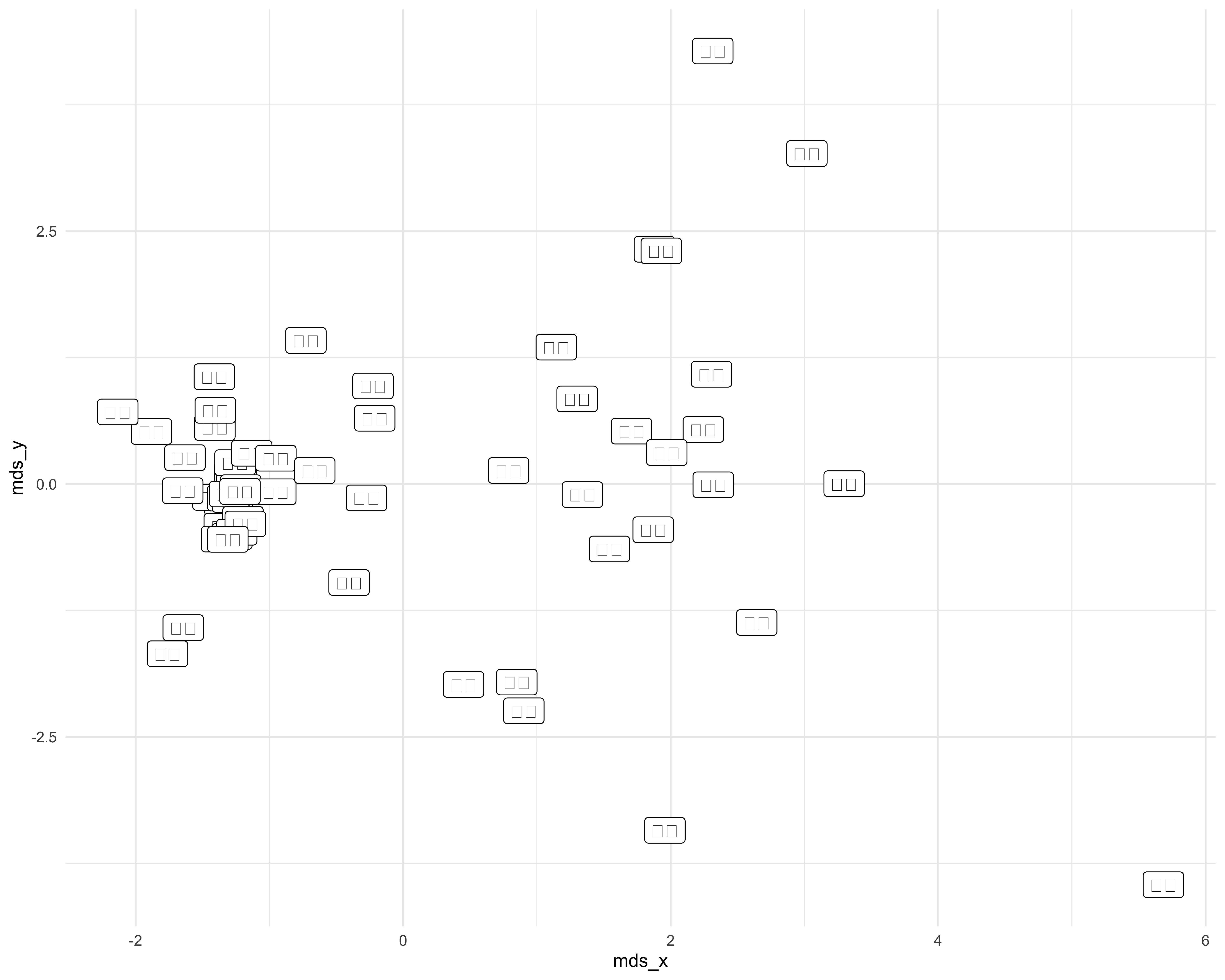

Hah…nice try. While the emoji look fine when you use head(), it’s not the same case when you try to plot them (from the poking around I did on stack overflow (see here) this has to do with your operating system/how you save the plot).

Behind the fancy emoji, this is what is lurking:

emoji_coords2 %>% pull(emoji)

##  [1] "\U0001f347" "\U0001f348" "\U0001f349" "\U0001f34a" "\U0001f34b"
##  [6] "\U0001f34c" "\U0001f34d" "\U0001f34e" "\U0001f34f" "\U0001f350"
## [11] "\U0001f351" "\U0001f352" "\U0001f353" "\U0001f95d" "\U0001f345"
## [16] "\U0001f951" "\U0001f346" "\U0001f954" "\U0001f955" "\U0001f33d"
## [21] "\U0001f336" "\U0001f952" "\U0001f344" "\U0001f95c" "\U0001f330"
## [26] "\U0001f35e" "\U0001f950" "\U0001f956" "\U0001f95e" "\U0001f9c0"
## [31] "\U0001f356" "\U0001f357" "\U0001f953" "\U0001f354" "\U0001f35f"
## [36] "\U0001f355" "\U0001f32d" "\U0001f32e" "\U0001f32f" "\U0001f37f"
## [41] "\U0001f358" "\U0001f35a" "\U0001f35d" "\U0001f364" "\U0001f368"
## [46] "\U0001f369" "\U0001f36a" "\U0001f370" "\U0001f36b" "\U0001f36c"
## [51] "\U0001f36e" "\U0001f36f" "\U0001f95b" "\U0001f375" "\U0001f376"
## [56] "\U0001f37e" "\U0001f377" "\U0001f37a"

Figuring out how to get emoji into a ggplot was quite the battle. I ended up spending a lot more time than I would like to admit getting the plot to look exactly how I wanted it to given the format of the original dataset. Although I didn’t end up using it because of of some compatability issues with this dataset, the emoGG package on github was super helpful when I was figuring out how to get this plot to work!

From looking at the emoGG package I learned that I could use Twemoji to grab the images that I wanted. I just needed to extract the last part of the unicode of each emoji to use to get the correct url. To do this, I used stri_escape_unicode() from the stringi package with str_replace() from the stringr package. Once I had this, I could create the appropriate urls for each emoji and pass that onto geom_image() from the ggimage package. In the end, this felt surprisingly simple but it took me quite a while to get to this solution.

emoji_coords2 <- emoji_coords2 %>% 
  # extract the code point
  mutate(code_point = str_replace(stringi::stri_escape_unicode(emoji), "\\\\U000", "")) %>% 
  # create image urls
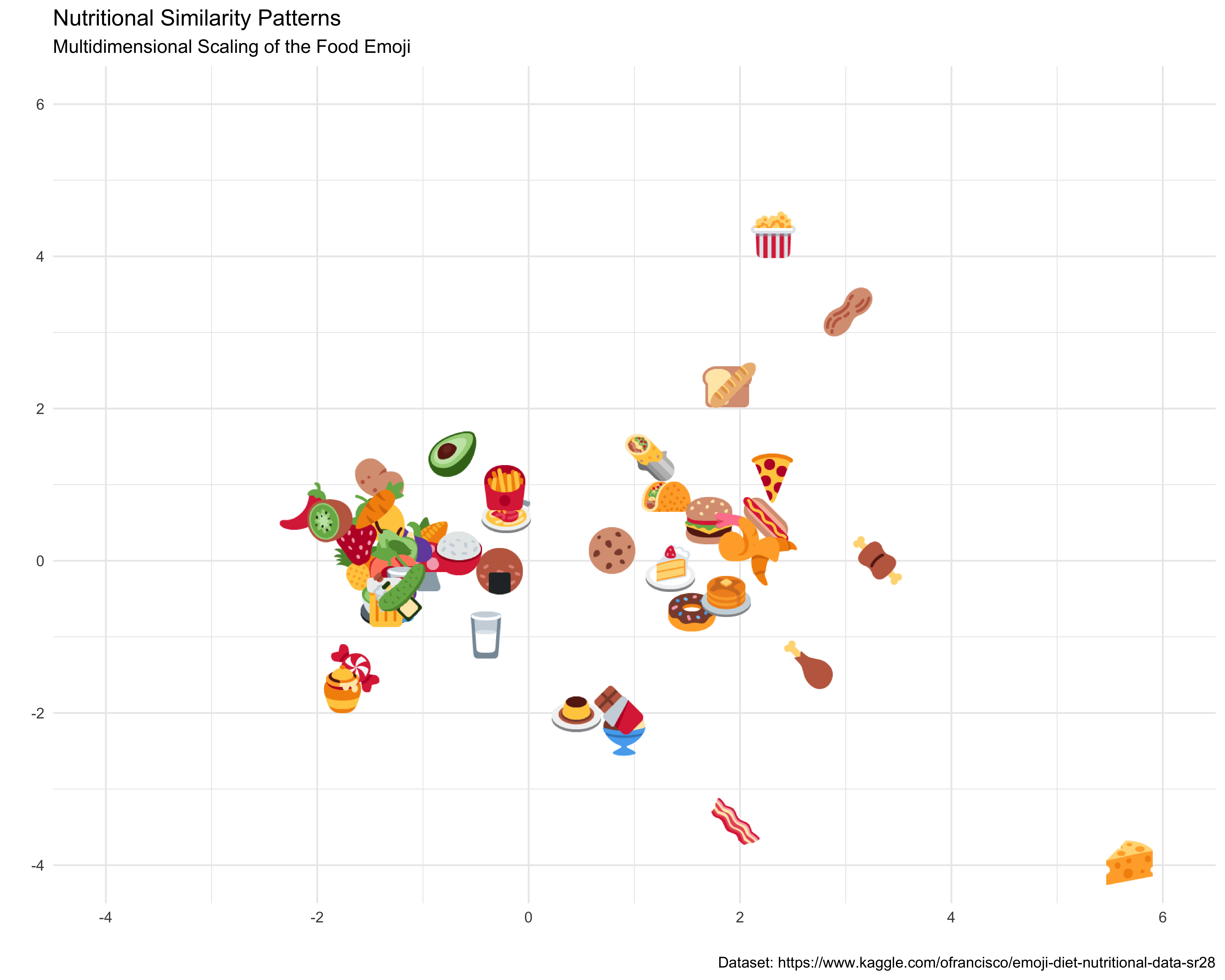
  mutate(img_url = map_chr(code_point, ~ str_glue("https://twemoji.maxcdn.com/2/72x72/", ., ".png")))

Finally….the plot!

ggplot(emoji_coords2, aes(mds_x, mds_y)) +
  geom_image(aes(image = img_url)) +
  theme_minimal() +
  labs(title = "Nutritional Similarity Patterns",
       subtitle = "Multidimensional Scaling of the Food Emoji",
       caption = "Dataset: https://www.kaggle.com/ofrancisco/emoji-diet-nutritional-data-sr28",
       x = "", y = "") +
  coord_cartesian(xlim = c(-4, 6), ylim = c(-4,6))